- PyBioProx Intro
- Installing and launching PyBioProx (Experienced Python Users)
- Installing and launching PyBioProx (Novice Python Users)
- Getting started guide (GUI)
- Getting started guide (Extensible Python Module)
- Image requirements
- Preprocessing Tips for Appropriate Object Detection
PyBioProx Intro
PyBioProx is a simple tool built in Python that analyses the relative proximity of fluorescent biomarkers in 2D or 3D microscopy images. For example, to analyse whether the distance between fluorescently labelled organelles or proteins (e.g. the distance between mitochondria and the nucleus) changes according to experimental parameters. PyBioProx generates perimeter distance (PD) measurments (Figure 1). A PD measurement is the shortest distance between a perimeter pixel of an object in one fluorescent channel (e.g. Channel 1) to the nearest fluorescent signal in another channel (e.g Channel 2). As described in our preprint, the mean of these measurements (PDmean) describes the proximity of the object in channel 1 to the fluorescent signal in channel 2. Taking the maximum (Hausdorff Distance) and the minimum (PDmin) PD measurement can also provide useful information however their use is discouraged for reasons discussed here.
PyBioProx is provided as an extensible Python module or as a GUI that can be run from the command line.
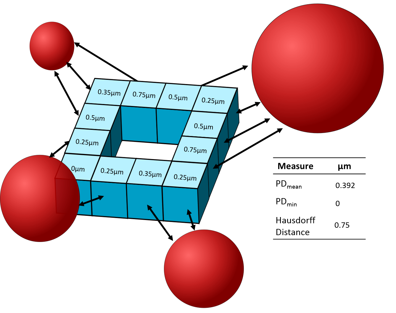 Figure 1 - An illustrative example in which a 3D (blue) object contains 12 perimeter voxels. The numbers within each
perimeter voexl show the PD measurement for each voxel relative to the red objects.
The smallest PD measurment represents the PDmin, the largest PD measurment represents
the Hausdorff Distance, the mean PD measurement represents the PDmean.
Figure 1 - An illustrative example in which a 3D (blue) object contains 12 perimeter voxels. The numbers within each
perimeter voexl show the PD measurement for each voxel relative to the red objects.
The smallest PD measurment represents the PDmin, the largest PD measurment represents
the Hausdorff Distance, the mean PD measurement represents the PDmean.
Installing and launching PyBioProx (Experienced Python Users)
-
Both the PyBioProx python module and GUI are distributed on PyPI.
-
To install the Python module, you can use pip as follows:
pip install pybioprox
- If you wish to install the optional graphical user interface (GUI) script, this may
be done by specifying the
guioptional extra:
pip install pybioprox[gui]
-
Once installed, the module can be invoked from the command line using:
python -m pybioprox <path_to_folder>, to run the analysis on all data files at the locationpath_to_folder -
If you have installed the GUI component or already have the required gui libraries, then you can also run
pybioprox_guidirectly from the command line.
Installing and launching PyBioProx (Novice Python Users)
1: The PyBioProx graphical user interface (GUI) requires Python to be installed on your computer. For ease of installation, we reccomend using the Anaconda distribution of Python. However more light-weight distributions of Python can also be installed. If you choose to not use the Anaconda installation, ensure that Python is added to the PATH and that a version of Python that is bundled with PIP (i.e. Python 3.4 or newer) is selected.
2 If using Anaconda, locate and open ‘Anaconda Prompt’. You will see something similar to the image below where (base) C:\Users\jdeed> is replaced with your username/location. Else, open ‘Command Prompt’ and launch Python by typing Python followed by Enter.
![]()
3 Type the following pip install pybioprox[gui] and press Enter. This will download the PyBioProx module alongside its GUI
and all of the necessary additional python modules that PyBioProx requires to function. You may have to confirm that you wish
to download these packages by pressing y followed by Enter.
You should see the following message Successfully installed PyBioProx(current version number)
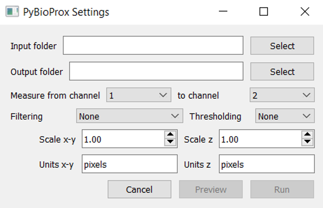
The GUI can then be launched by typing pybioprox_gui follwed by Enter. The following window should appear:
Getting started guide (GUI)
We have provided two images sourced from the Colocalisation Benchmark Source (CBS) that can be downloaded by clicking this link to follow along with this guide. CBS provides images with known (ground-truth) levels of colcalistion, we have included two images from CBS dataset 2 with ground-truth colocalisation values of 0 (CBS001RBM__0percent_colocalisation.tif) and 90 % (CBS0010RBM__90percent_colocalisation.tif). Below is a follow-along tutorial using these images.
1: Launch the PyBioProx GUI
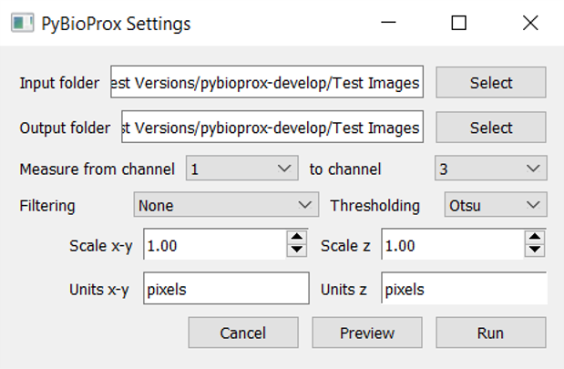
2: Select the (unzipped) ‘CBS Images’ folder as the input.
3: Select an output folder where you want the results to be saved.
4: In the test CBS images, Channel 1 contains ‘Red’ objects, ‘Channel 2’ contains nothing and ‘Channel 3’ contains ‘blue objects’. To measure the PDmean distances of red objects to blue objects, select ‘Measure from channel 1 to channel 3’ using the drop down menus.
5: PyBioProx currently only provides a limited number of preprocessing operations. A gaussian filter (sigma 3) can be performed on images if required by selecting from the ‘Filtering’ dropdown menu. If any other preprocessing is required, this should be performed (e.g. in Python or ImageJ) before loading the images into the PyBioProx GUI. The CBS test images do not require preprocessing, so leave the ‘Filtering’ parameter blank.
6: These sample images have not previously been binarised. Therefore, a thresholding algorithm must be used to identify regions with and without fluorescent signal. Currently two thresholding algorthims are offered. Both algorithms work reasonably well on these images. Select the ‘Otsu’ thresholding algorithm.
7: PyBioProx makes distance-based measurements. These can either be in units of pixels/voxels, or in real-world measurements e.g. micrometeres, if the dimensions, of the pixels or voxels are known. ‘Scale x-y’ describes the size of the pixel in the X and Y axes while ‘Scale z’ provides the distance between each Z-slice (often referred to as ‘step size’). NB. an easy way to identify pixel/voxel dimensions is to open images in Fiji and press ‘i’.
The CBS sample images that we are using in this tutorial are 2D with no accompanying distance metadata. As such, we will leave the units as pixels and the Scale as 1.
The settings should now look like the below:
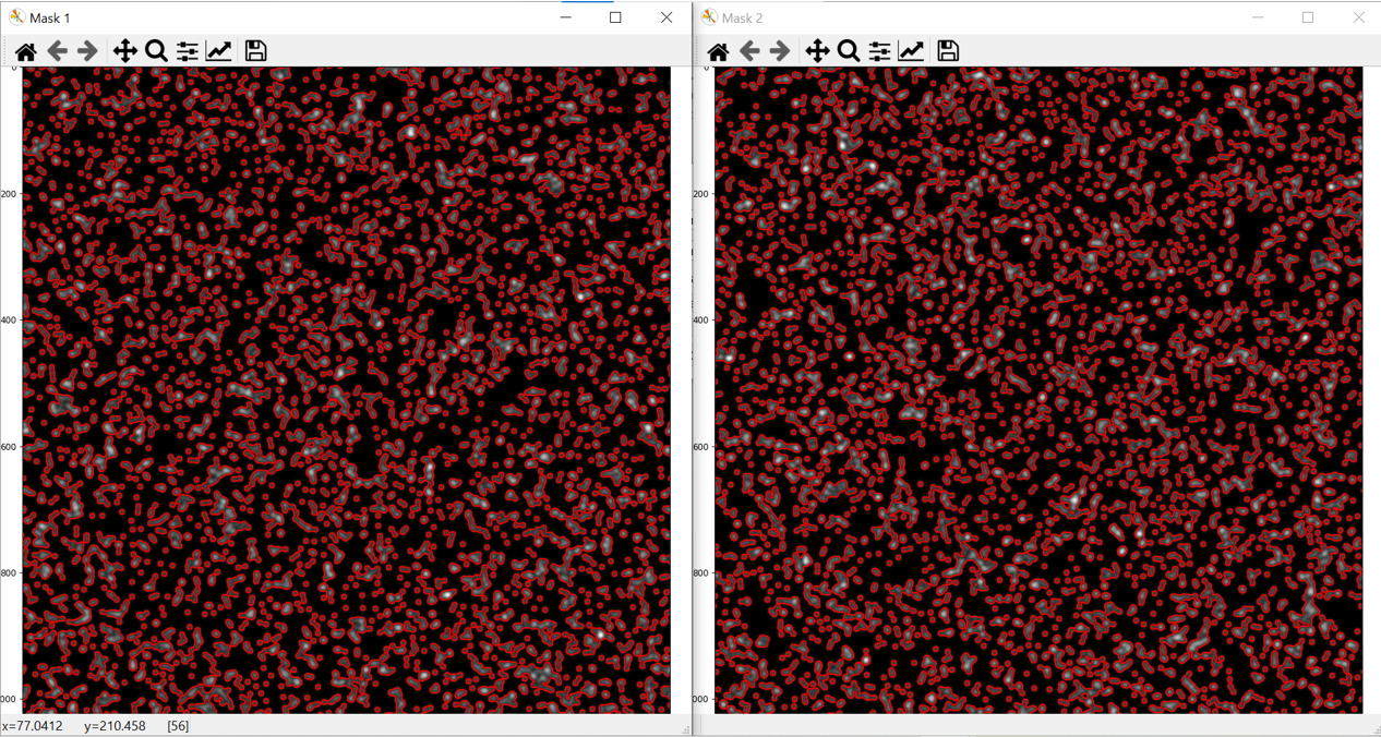
8: Press ‘Preview’. This will select the first .tif file in the folder, perform the filtering operation, binarise the image using the selected thresholding algorith and detect objects. Two images will then appear as shown below.
-
These images show an overlay of the perimeter of the objects that PyBioProx has detected ontop of the original image. Mask1 = overlay of ‘channel to be measured from’, Mask2 = overlay of ‘channel to be measured to’
-
If the image is a Z-stack, the preview function will show object detection on the middle slice of the Z-stack.
-
It is essential to always check that the object-detection is appropriate. I.e. is PyBioProx detecting objects of the size and shape that you expect. If PyBioProx is not correctly identifying objects, this suggests that either the thresholding algorithm or preprossessing steps that have been used are not optimal. For tips about how to optimise preprocessing for better object detection click here.
-
To try different PyBioProx parameters and see the effect on object detection, save and close the preview ‘mask’ images, change the parameters and press ‘Preview’ again.
9: Once you are happy with the object detection, click ‘Run’.
10: PyBioProx will then process all the .tif images in the folder.
- PyBioProx will create two .png image files (for mask 1 and 2) showing object detection (middle slice if analysing a Z-stack image) .png files will be saved to the input folder.
- For each image, PyBioProx will create two .csv files named ‘distance_table_your-filename’ and ‘stats_table_your_filename’.
- The ‘distance_table’ files show all PD measurements for each detected object. PD measurements from the same object appear on the same row.
- The ‘stats_table’ files are generally more useful. They provide the PDmean, PDmin and Hausdorff Distance for each object in the analysed image. PD measurements from the same object appear on the same row.
- Averaging the PDmean values then identifies the
average proximity of red objects to blue objects in each image. Using the parameters in this example:
- The average red object in the 0 % CBS image has a PDmean proximity to blue objects of 3.56 pixels.
- The average red object in the 90 % CBS image has a PDmean proximity to blue objects of 0.64 pixels.
Getting started guide (Extensible Python Module)
- PyBioProx can be launched directly from the command line using the following command:
python -m pybioprox <path_to_folder>, to run the analysis on all data files at the location path_to_folder
- If however, you wish to use PyBioProx within a Python script (and to have control over the parameters of PyBioProx
without using the GUI), then you must import the
mainmodule from PyBioProx as follows:
import pybioprox
from pybioprox import main
- PyBioProx analysis can then be used with the main.main() function:
main.main(filepath, output_folder, channel1_index, channel2_index, filter_method, threshold_method, distance_analyser, scales, units)
Parameters
filepath : str Location of folder containing .tif files
output_folder : str: Location of output for mask images and .csv files containing measurements
channel1_index : int:
Channel to be measured from (default = 0)
channel2_index : int:
Channel to be measured to (default = 1)
filter_method : str:
Preprocessing method (the only method currently supported is 'gaussian (sigma 3px)') (default = 'none')
threshold_method : str:
Currently available thresholding methods are 'otsu' or 'li', default = 'none'
distance_analyser : str:
Method of analysis, not changeable 'edge-to-edge'.
scales : tuple:
Size of pixels/voxels (XY distance, Z distance), default = (0.08,0.75)
units : tuple:
Units of measurement, default = ('um','um')
max_num_objects int:
The largest number of objects that can be detected before the image
is aborted, default = 10000
Image requirements
- PyBioProx currently only functions with images saved in the .tif format, more information on file types can be found here.
- Batch conversion of other file types to .tiffs
- Images must be composites (multichannel images)
Preprocessing Tips for Appropriate Object Detection
-
Without appropriate object-detection, PyBioProx will not produce meaningful data! For this reason, when analysing large datasets, it is essential to optimise preprocessing and thresholding steps on a representative sample of images. It is also essential to check through the ‘mask.png’ images produced (step 7 in GUI tutorial section) for all analysed images.
-
PyBioProx detects objects first by thresholding the image, to create binary images in which pixels are either ‘on’ (pixel value = 1) or ‘off’ (pixel value = 0). Connected ‘on’ pixels are then ‘labelled’ as objects using the
scipy.ndi.labelmodule. -
PyBioProx allows for images to be thresholded using either ‘Otsu’ or ‘Li’ thresholding algorthims. Alternatively, images can be thresholded in another program (e.g. ImageJ) and the resulting binary image analysed in PyBioProx (thresholding program = ‘None’).
-
Different thresholding algorithms will be appropriate for different images, try opening your images in ImageJ and trying a few out, if you find one that works well (but isn’t provided in PyBioProx), then one option is to batch threshold your images in ImageJ and then process the resulting binary images in PyBioProx.
-
If no thresholding algorithm appropriately identifies positive and negative fluorescent signal, this indicates that preprocessing is required
-
If small regions of ‘noise’ are being erroneously identified as objects by PyBioProx, filtering operations such as a gaussian filter may help to ‘smooth out’ this noise. A gaussian filter with a 3px kernal can be applied in PyBioProx. This is currently the only preprocessing operation offered in PyBioProx, other filtering operations must be applied to images prior to analysis in PyBioProx.
-
If object detection is not descrete enough, i.e. the objects detected appear to be larger than they should be, then preprocessing operations such as an unsharp mask, or a top-hat filter, can be employed to enhance the most salient features of the image.